Flip-flop and Latch : Internal structures and Functions

The flip flop is the most commonly used sequential element in any ASIC design, especially the D-type flip-flop. In the D flip flop, the D indicates delay, which means the output is a delayed version of input D.  Whereas a latch is the simplest and a basic sequential element. In general, there are two latches used to make a flip flop. the flip-flop is sensitive to clock edge and the latch is sensitive to clock level. The following section will explain the internal structure and operation of flip flops and latch. In this article, we will limit our discussion to only d type flip flops and d type latch which are most common in ASIC design. 

Schematic of the latch and flip-flop

The simplest design latch and flip-flop both are having 3 pins, One input data pin (D), one input clock/enable pin (CP/E) and, one output pin (Q). There could be a set and reset pins also but here for simplicity we are not including those in our discussion. The symbolic representation of a latch and a flip flop has been shown in figure-1.

Figure-1: Symbolic representation of Latch and flip-flop

In figure-1, the symbol of a posotive level sensitive d-latch and a positive edge triggered d flip-flop has shown. In negative latch and flip-flop only a dot appears before the E/CP pin. At a high level, we can think that latch and flip flop in terms of 2:1 multiplexer. A latch can be realized using a 2:1 multiplexer whereas to realize a flip flop, two multiplexers are required. Figure-2 showing the architecture of positive level sensitive d-latch and a positive edge triggered flip flop in terms of multiplexers.

Figure-2 : A positive d-latch and flip-flop using multiplexer

In a positive level sensitive latch the output is fed to I0 input of multiplexer as shown in figure-2. In same way in a negative level sensitive d-latch the output Q is fed back to input I1. A positive edge triggered d-flip flop is made of two negative level sensitive d-latch connected back to back. In case of negative d flip flop two positive level sensitive d-latch would be required. If we dive deep inside the multiplexer and go to the transistor level, we will find the transistor level schematic of a positive level sensitive d-latch and positive edge triggered d flip-flops as shown in figure -3.

Figure-3.a : A positive level sensitive d-latch using transmission gates

Figure-3.b: A positive edge triggered d flip-flop using transmission gates

A 2:1 multiplexer is made of two transmission gates and a transmission gate is made using a pMOS and an nMOS transistor as shown in the above figure. A latch is having two transmission gates in which the input of one transmission gate is connected to the output. A flip flop is made of two latches (that is four transmission gates) connected back to back as shown in figure-3. From the above figure, it is clear that a flip flop is having more transistors (double) as compare to a latch and hence a flip flop is having double the area as compared to the latch. The understanding of the working of latch and flip-flop is the most important part which will be discussed in the next section.

Working of a d- latch

The working of a positive level sensitive d-latch only is discussed here with the help of input and output waveform. The working of flip-flop will be discussed in the next section.

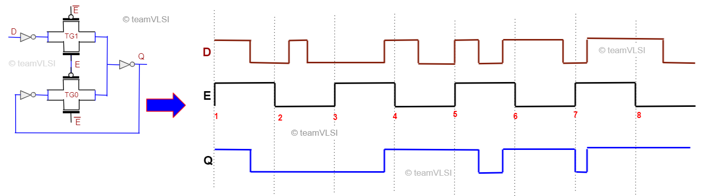
Figure-4: Input-Output waveform of latch

There are two transmission gates are used in a d-latch. In case of a positive level sensitive d-latch the output is feedback to the input of TGO transmission gate. Transmission gates are made of a nMOS and a pMOS as shown in above figure and it is being controlled by the enable signal E which is actually the clock signal. When the enable signal is high, the nMOS and pMOSof TG1 is in on state and at the same time, both transistors of TG0 are in off state and vice-versa happens when the enable signal is low. There is a direct path established from pin D to pin Q when the Enabe signal is high and it is called latch is in transperent state. But when enable signal goes low, TG1 gate is in off state and a feedback loop is established between Q to input of TG0 which insures that there is no change in output Q irrespective of changes in input pin D, which is termed as latch state. Figure-5 shows when the latch is transperent and when it is latched through the waveform. 

Figure-5: Working of a positive level sensitive d latch.

The working of a positive level sensitive d-latch is straight forward, it keep passing the input D to Q when its enable signal E is high and and it keep the output Q unchanged when enable signal is low. Same can be seen in figure-5, only output changes when input changes and enable signal is high.

Working of a d flip-flop

In a positive edge triggered d flip flop, there are two negative level sensitive d latch connected back to back and the second latch is having inverted enable signal as compare to first latch. This inverted enable signal to second latch makes sure that both the latch  never goes transperent or latched state simultaneously. A typical input output waveform has shown in figure-6 for better understanding.

Figure-6: Input output waveform of a positive d flip-flop

Lets consider the the case when the clock signal is low, the first latch is transperent and input D is transmitted up to QM point. But at the same time second latch will be in latched state because it gets inverted clock signal so the output Q is latched with QM. There is no chance the outupt Q will get changed in this duration.

The next moment when clock signal transits from low to high, the first latch will go from transperent mode to latched mode and second latch will go from latched mode to  transperent mode. So during the clock transition from low to high, whatever signal is sampled at QM previously gets transferred to the output Q.

The next moment when clock signal goes to high, there is not transfer of input signal D anymore and Wahtever signal previously samples at QM will be available at output Q.

The next moment when the clock signal transits from high to low, first latch will trasit from latched to transparent mode and second latch will transit from transparent to latche mode. So at this edge of clock transition there will be no change in output.

The operation of positive d flip flop can be summarized as, the output changes only at the rising clock edge and at this moment input D is trasfered to output Q and all other moment output is remain unchanged. So it is better in terms of avoid glitch as comapare to latch but more in area and more prone to process variation. For detailed operation and comparison please watch this playlist.

Thank you.

Tie Cells in Physical Design

The tie cell is a standard cell, designed specially to provide the high or low signal to the input (gate terminal) of any logic gate. The high/low signal can not be applied directly to the gate of any transistors because of some limitations of transistors, especially in the lower node. The limitation will also be discussed along with the schematic and operation of tie cells in this article. We will discuss the following sub-topics in this article.

• Need of tie cells
• Schematic of tie cells
• The function of tie cells
• Placement of tie cells

Need of tie cells:

In the lower technology node, the gate oxide under the poly gate is a very thin and the most sensitive part of the transistor. We need to take special care of this thin gate oxide while fabrication (associated issue is antenna effect) as well as in operation too. It has been observed that if the polysilicon gate connects directly to VDD or VSS for a constant high/low input signal, and in case any surge/glitch arises in the supply voltage it results in damage of sensitive gate oxide. To avoid the damages mentioned above, we avoid the direct connection from VDD or VSS to the input of any logic gates. A tie cell is used to connect the input of any logic to the VDD or VSS.

Figure-1: Need of tie cell

There are two types of tie cells.

• Tie-high cell
• Tie- low cell

As the name suggests, the tie-high cell's output is always high and the tie-low cell's output is always low.  

Schematic of tie cells:

The tie cell has no input pin and only one output pin. The output of the tie-high cell is always high and the output of the tie-low cell is always low and it is the glitch-free output that connects to the input of any logic gates. The schematic of tie high cell and tie-low cell is shown in the figure-2.

Figure-2: Tie-high and tie-low cells

In the tie-high cell, the drain and gate of nMOS are shorted together and connected to the gate of pMOS, and output is taken from the drain of pMOS. Whereas in the tie-low cell the drain and gate of pMOS are shorted together and connected to the gate of nMOS and output is taken from the drain of nMOS. The function of these schematics is explained in the next section.

Function of tie cells:

Both tie-high and tie-low cells have similar working. Here working of the tie-high cell is explained. A similar logic can think for tie-low cell. From figure-2 tie-high cell, the drain and gate of nMOS are shorted.

So Vg = Vd
==> Vgs = Vds
Therefore, Vds > Vgs -Vt

This shows that the nMOS will always be in the saturation region. The configuration of MOS where drain and gate are shorted is popularly known as a diode-connected transistor. And when nMOS is behaving like a diode here, the gate of pMOS is always low and so pMOS is always in on state. When pMOS is in on state its drain which is output will always be high.

Similarly, for the tie-low cell, the pMOS is always in saturation region so the gate of nMOS is always high and hence the drain of nMOS will always be at the low logic.

One more important thing is here that the sudden spike in VDD or VSS will be not propagated to the output of the tie cell.

Placement of tie cells:

Tie cells are not present in the synthesized netlist and not placed in the initial placement of the standard cells. Tie cells are inserted in the placement stage and more specifically at the final stage of placement. Where ever netlist is having any pin connected to 0 logic or 1 logic (like .A(1'b0) or .IN(1'b1), a tie cell gets inserted there. Click here to read more about the placement stage and the order where the tie cell get inserted in the placement stage.

Thank you.

Integrated Clock Gating (ICG) Cell in VLSI

 Low power ASIC design is the need of the hour, especially for hand-held electronics gadgets. In all hand-held products, the customer demands more battery life. This could be possible only if our SoC (System on Chip) inside the gadget consumes lesser power. There are various low-power design techniques that are being implemented the reduce the power consumption of application-specific integrated circuits (ASIC). The clock gating technique is one of the widely used techniques for low power design. Integrated Clock Gating (ICG) Cell is a specially designed cell that is used for clock gating techniques. In this article, we will go through the architecture, function, and placement of ICG cells.

Why ICG Cell?

ICG cell basically stops the clock propagation through it when we apply a low clock enable signal on it. This phenomenon is termed clock gating. We use the ICG cell to stop the clock signal propagation to a big group of logic cells when the group is not required to operate. This is done through a clock enable signal generated internally in the block and applied to the EN pin of the ICG cell.  We know that the total power consumption of an SoC is the sum of dynamic power and static power. The clock tree is a major contributor to dynamic power as the clock signal has maximum switching activities. The ICG cell allows to stop the clock signal propagation beyond it and it helps to reduce dynamic power consumption in the design.

The architecture of ICG Cell:

There are various ways to implement the clock gating techniques and there are many architectures of ICG cells also. Here the most common architecture is Latch-AND based ICG cell. 

Figure-1: Latch-and based ICG Cell

Prevention of glitches is one of the qualities of ICG cells. The latch-and gate based ICG cell is good on that front and that's why this architecture of clock gating circuit is used widely. There are various architectures of ICG cells but we are limiting our discussion to only this architecture in this article. 

The function of ICG Cell:

Figure-2: Waveform of ICG Cell

As shown in the above figure it provides a glitch-free clock gated output. and passed the clock single only when the enable signal is high and stop the clock propagation when enable signal is low. 

Why not only AND gate as a clock gating?

The issue with the AND gate as clock gating is, it can not provide a glitch-free output whereas a glitch-free clock wave is highly desired. 

Figure-3: AND gate as a clock gater

If there is a transition in clock enable signal when the clock signal is low, there is no effect on the gated clock. But if there is a transition in clock enable signal when the clock signal is high, there will be a glitch in the gated clock. To suppress such glitches, latch-and gate based ICG cell is preferred. 
The placement of ICG cells will be discussed in the next article.

Thank you

Important questions from Readers:

1. Why do we use Latch in ICG why not flip flop? (by Ramcharan)

Ans:

1. As we not that flip flop will capture the data only at the edge of the clock signal so any data change between one active edge to next active edge will not be captured.

2. If we use -ve edge FF the setup timing requirement for FF to ICG will be half cycle which is again difficult to meet in case of ICG placed near the sink.

Here is a waveform showing the differences in operation.

Multi Bit Flip Flop Vs Single Bit Flip Flops

In modern ASIC design use of multi-bit flip flops (MBFF) has increased due to its various promising advantages of MBFF over single-bit flip flop (SBFF). Traditionally we study only a single-bit flip flop in our academics. So it becomes important to understand the design of multi-bit flip-flops, how it works, and what are the advantages/disadvantages of multi-bit flip-flops over single-bit flip-flops.

Why Multi-bit Flip Flops?

Multi-bit flip flop has many advantages due to its architecture over the single-bit flip flop. There are many recent research publications also which show these facts with proper statics. We also witness these advantages while place and route (PnR) implementation. Here I  would like to explain the basic facts of MBFF in a simple way without any detailed statics. The exact statics can be referred from any recent research publications. The main advantages of multi-bit flip flop are as follows and that's why MBFF is used widely now a day. 

1. Area reduction
2. Power reduction (promising for low power designs)
3. Better clock skew control
4. Timing improvement

So we can say that it improves the area, power, and timing. The reason for these advantages will be explained in the next section.

Multi-bit Flip Flop Architecture:

All the advantages of multi-bit flip-flops are due to their architecture. A single-bit FF and a 2-bit MBFF schematic have shown in the figure-1. A similar architecture can imagine for higher bit MBFF also.

Figure -1: Multi-Bit Flip Flop

One can notice that the inverter count reduces when we use the multi-bit flip flop as compare to the single-bit flip flop. The effect of this reduction is more visible when we use bigger MBFF. A comparison of inverter count in SBFF and MBFF has shown in figure-2.

Figure-2: Number of Inverters used in SBFF and MBFF

Instead of 16 inverters inside 8 single-bit flip flops, there are only 2 inverters used inside a 16-bit flip flop. A  schematic of 8-bit MBFF has shown in figure-3.

Figure-3: 8-bit MBFF

As the number of inverters reduced in the case of MBFF, it saves the clock power and area. There is no change in the operation of flops after MBFF conversion. Now let's discuss the mechanism of how PnR tools convert the SBFFs into MBFFs.

MBFF conversion: 

Figure-4: Placement of flops before MBFF conversion

Figure-5: Placement of MBFF after conversion

Figures 4 and 5, show how the conversion of SBFF into MBFF. Figure-4 is showing the scenario before MBFF conversion is done and figure-5 shows the scenario after MBFF conversion. In figure-5, we can see that instead of 8 different SBFF only one 8-bit MBFF is used. So MBFF is generally bigger in size and having multi-row height standard cell. 

PnR tools have algorithms to convert SBFF into MBFF. The tool picks the equivalent MBFF available in the standard cell library and performs the conversion with respect to the user input provided for conversion. This conversion happens in the placement stage.

If we talk about the Cadence Innovus tool, we have a command 

setOptMode -multiBitFlopOpt true 

Which enables PnR tools for multibit flop conversion. By default, this conversion is disabled in the tool. There are many such commands in the tool which can be explored further.

 

Thanks.

Spare Cells in Physical Design

Once a chip is fabricated and if any functionality issue is found in the chip or some functionality enhancement is required in the next fabrication. This might be a very challenging task without spare cells. But with the help of pre-placed spare cells, these changes can be done very easily. In this article, we will discuss the spare cells in physical design.  

Spare cells:

Spare cells generally consist of a group of standard cells mainly inverter, buffer, nand, nor, and, or, exor, mux, flip flops and maybe some specially designed configurable spare cells. Ideally, spare cells do not perform any logical operation in the design and act as a filler cell only. A group of spare cells is shown below. 

The inputs of spare cells are tied either VDD or VSS through the tie cell and the output is left floating. Input can not be left floating as a floating input will be prone to get affected by noise and this could result in unnecessary switching in space cells which leads to extra power dissipation.

Use of Spare cells:

Spare cells enable us to modify/improve the functionality of a chip with minimal changes in the mask. We can use already placed spare cells from the nearby location and just need to modify the metal interconnect. There is no need to make any changes in the base layers. Using metal ECO we can modify the interconnect metal connection and make use of spare cells. We only need to change some metal mask, not the base layer masks.

For example, suppose in the above circuit we need to replace the last OR gate in the middle part of a circuit with an EXOR or an AND gate, we can reconnect the spare cell placed near this with metal ECO only.

Placement of Spare cells:

Spare cells can be added either by the netlist or by PnR tool command (or GUI too). In Physical design, we prefer to add the spare cells using tool command. These cells are added before the placement of standard cells throughout the design. The way of adding spare cells for Innovus and ICC tool has been explained below.

Innovus tool:

ICC tool:

Advantage and disadvantage of Spare cells:

Advantage:

Reusability: 

There is only change in some metal and via masks, so base layers mask can be reused in chip fabrication.

Flexibility: 

Small changes can be done in the design very easily.

Cost and Time saving: 

We need only a few interconnect mask for a new design, which save lots of manufacturing cost for new chip fabrication. And using metal ECO we do not need to run full design cycle and therefore save design time.

Disadvantage:

Leakage Power: 

Spare cells increase the leakage power dissipation in the design.

Area: 

Spare cells cost extra area overhead in the design.

Thank You.

DeCap Cells in Physical Design | Use of Decap Cells in PD

Decap cells are basically a charge storing device made of the capacitors and used to support the instant current requirement in the power delivery network. There are various reasons for the instant large current requirement in the circuit and if there are no adequate measures have taken to handle this requirement, power droop or ground bounce may occur. These power droop or ground bounce will affect the constant power supply and ultimately the delay of standard cells may get affected. To support the power delivery network from such sudden power requirements, decap cells are inserted throughout the design. In this article, we will discuss the structure and layout of decap cells, need of using decap cell and placement of decap cells.

Schematic and layout of Decap cell:

There could be various ways to make capacitors out of MOS transistors but the must widely used structure is shown in the figure-1. 

Figure-1: MOS Capacitances and Decap cell schematics

Figure-1(a) shows the various capacitances inside the MOS transistor and it if we connect the source, drain and body terminal together then all these capacitance will configured as a parallel capacitance as shown in figure-1(b) and a single equivalent capacitance as shown in figure-1(c). Figure-1(d) shows a decap capacitor schematic using a pMOS and an nMOS transistor. From this schematic, we can say that the capacitance due to nMOS and pMOS will be in parallel and get added to form a big capacitor. Figure-2 shows the layout of a simplest decap cell.

Figure-2: Layout a decap capacitor 

Source and drain of pMOS transistor shorted together and connected to VDD and the Gate is connected to VSS. Similarly, the source and drain of the nMOS transistor are connected to the VSS and gate is connected to VDD.

Use of  Decap cell:

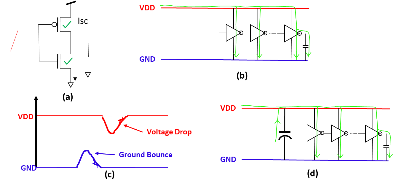
In the operation of CMOS logic, there is a region of input transition where both the nMOS and pMOS is conducting together as shown in figure-2(a). A large short circuit current Isc will flow for that instant. If a large number of such cells are placed together and switching together, a large current will be required as shown in figure-2(b). This large current requirement may drop the VDD or may increase the ground voltage which is called voltage droop or groud bounce as shown in figure-2(c).

Figure-2: Need of Decap cell

Voltage droop or ground bounce may result in the change in the delay of connected standard cells. As the delay is proportional to the supply voltage. Change in delay may further affect the timing of design and if the supply voltage drop is high, the functionality of the standard cell may get affected. So to support the power delivery, we add the decap cells. Decap cells work as charge reservoirs and support the power delivery network and make it robust as shown in the figure-2(d). 

Placement of  Decap cell:

Decap cells are placed generally after the power planning and before the standard cell placement, that is in the pre-placement stage. These cells are placed uniformly throughout the design in this stage. Decap cells can also be placed in the post route stage also if required. 

The only problem with decap cells is that these are leaky and increases the leakage power of design, so must be used judiciously. 

Thank you.

End Cap Cells in VLSI | Boundary Cells in VLSI

There are high chances to get damaged the gate of standard cells placed at the boundary during the manufacturing of chip. To prevent such damages at the boundary we have a special kind of cell in the standard cell library is called end cap cell or boundary cell. Boundary cell not only protects the gate damage at the boundary, but it also serves many other purposes. In this article, we will discuss the need for boundary cell placement, the structure and placement of boundary cells.

Where to place End Cap / Boundary Cells:

The end cap cell or boundary cell is placed at both the ends of each placement row to terminate the row. It has also been placed at the top and bottom row at the block level to make integration with other blocks. Some standard cell library has also corner end cap cells to place the corner of the block. Boundary cells have fixed attribute, therefore these cells can not be moved during the optimization. A typical placement of end cap cells at the end of the row has shown in figure-1. 

Figure-1: Placement of end cap cell at the end of rows

Why need to place End Cap / Boundary Cell?

The end cap cells are placed in the design because of the following reasons:

• To protect the gate of a standard cell placed near the boundary from damage during manufacturing.
• To avoid the base layer DRC (Nwell and Implant layer) at the boundary.
• To make the proper alignment with the other block.
• Some standard cell library has end cap cell which serve as decap cell also.

Layout of end cap / boundary cell:

The boundary cell is a physical-only cell, has no logical functions and therefore these cells are not a part of the netlist.  Boundary cells have mainly Nwell layer, implant layers, and dummy poly layer and metal rails as shown in the figure-2. 

How to place:

Boundary cells are placed just after the macro placement and site row creation. Boundary cell is placed before the placement of standard cells and therefore it is called a pre-placed cell. End cap cells cab be added using GUI interface or through the tool commands. Commands to add the endcap cells in Innovus and ICC tools have given below.

For Innovus tool:

setEndCapMode -reset

setEndCapMode -rightEdge <CellName> -leftEdge <CellName> -topEdge <CellName> -bottomEdge <CellName>  -rightTopEdge <CellName> -rightBottomEdge <CellName> -leftTopCorner <CellName> -leftBottomCorner <CellName>

addEndCap -prefix <name>

verifyEndCap -report <reportName>

For ICC tool:

insert_boundary_cell

 

For details of these commands and related switches refer to the tool's command man page.

Thank you.

Well Tap Cells in Physical Design

Well tap cells (or Tap cells) are used to prevent the latch-up issue in the CMOS design. Well tap cells connect the nwell to VDD and p-substrate to VSS in order to prevent the latch-up issue. There is no logical function in well tap cell rather than proving a taping to nwell and p-substrate therefore well tap cell is called a physical-only cell. In this article, we will discuss the structure of well tap cell, the requirement of well tap cell and how to place them in the physical design flow.

Well Tap Cell:

Well tap cells having no logical functions, it has only two connections.

• nwell to the power supply (VDD)
• p-substrate to the ground (VSS)

A typical structure of well tap layout has shown in figure-1. Well tap cell has no input and output pins, therefore it is called a physical-only cell.

Figure-1: Layout of well tap cell

Why Well Tap Cell:

Early days there was no concept of well tap cell, Standard cells were designed in such a way that each standard cell had nwell to VDD and p-substrate to VSS connection within the standard cell. But such a standard cell design had consumed more area and to save the area, later a concept of Tapless cell has evolved. In a tapless cell, there are no well taping inside the standard cell, well taping is provided by a separate standard cell which is called a well tap cell. So well tap cell is a part of a tapless standard cell library. Figure-2 shows the structure of a traditional standard cell and a tapless standard cell.

Figure-2: Traditional and Tapless standard cell structure

Well tap cells are used to prevent the latch-up issue in design. how it prevent, has been explained in the article "latch-up prevention in CMOS" in this blog. 

Placement of  Well Tap Cells:

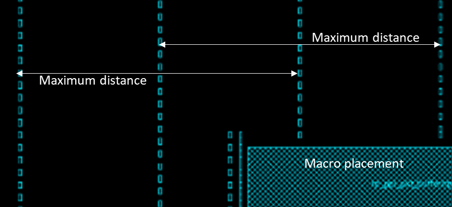
Well tap cells are placed after the macro placement and power rail creation. This stage is called the pre-placement stage. Well tap cells are placed in a regular interval in each row of placement. The maximum distance between the well tap cells must be as per the DRC rule of that particular technology library. A typical placement of well tap cells is shown in figure-3. 

Figure-3: Well tap cell placement

Well tap cells are generally placed in a straight column in the alternate row as shown in figure and such a pattern is called checkerboard pattern to provide maximum coverage for well tap. If a macro comes in the path of vertical columns, then the placement of vertical column shifted alongside macro as shown in the figure. 

This placement is performed using the PnR tool command. For ICC and Innovus tool following command have used to place the well tap cells.

For Innovus tool:

set_well_tap_mode -rule <> -bottom_tap_cell <cellName> -top_cell_name <cellName> -cell <> 

addWellTap  -cell <cellName> -cellInterval <maxGap> -prefix <prefixName> -checkerBoard -fixedGap

verifyWellTap -report <reportName>

For more details refer UG of Innovus tool.

For ICC tool:

add_tap_cell_array -ignore_soft_blockage true -master_cell_name $tapCell –distance $tapPitch -connect_power_name VDD -connect_ground_name VSS -respect_keepout -pattern stagger_every_other_row -tap_cell_identifier WELLTAP 

Thank you!

Standard Cell Library for ASIC Design

Standard cell library is an integral part of ASIC design flow and it helps to reduce the design time drastically. Standard cells used in the ASIC design is a part of a standard cell library along with some other file sets. In this article, we will discuss the important content inside the standard cell library and its uses.

Standard Cell Library:

Standard cell library is a collection of well defined and pre-characterized logic cells with multi-drive strength and multi-threshold voltage cells in the form of a predefined standard cell layout. It also contains a number of physical only cells and a set of library files required by Place and Route (PnR) tool for automatic placement and routing (APR).

Pre-characterization: 

Before including a standard cell into standard cell library, the cells are gone through schematic design, simulations followed by Symbol creation, layout design (as per standard cells layout rules), physical verifications, abstraction, extraction and characterization. So the cells available in standard cell library are free from any DRC violations, well-characterized and suitable for PnR tool for automatic placement and routing.

Multi-drive strength cells: 

A low drive strength cell will require less power and area but having more delay and more transition time whereas a high drive strength cell can drive a larger number of cells and having a fast transition. So as per the requirement, a PnR design engineer chooses the drive strength of cells to optimize the area, power and performance.

Multi-Vt cells: 

A low threshold voltage (LVT) cell will have a lesser delay but higher leakage power as compared to a high threshold voltage (HVT) cell. So as per the requirement of timing and power a PnR engineer uses HVT and LVT cell to balance the power and timing of the design. There is no difference in the area on multi-Vt cells. A modern standard cell library contains generally ULVT, LVT, SVT, HVT types of cells in which Vt is in increasing order.

Physical only cells: 

In physical design, We need to add a variety to standard cells to mitigate various effects and manufacturing issues. These cells do not have any logical functions. For example to overcome the latch-up issue we need to add well tap cells. Decap cells, endcap cells, antenna cells and filler cells are the example of such cells.  

In the next section, we will discuss various cells collection and standard cells library and the set of important files.

Cell Collections:

In general, a standard cell library contains the following types of cell:

• All basic and universal gates (like AND, OR, NOT, NAND, NOR, XOR etc)
• Complex gates (like MUX, HA, FA, Comparators, AOI, OAI etc)
• Clock tree cells (like Clock buffers, clock inverters, ICG cells etc)
• Flip flops and latches
• Delay cells 
• Physical only cells
• Scannable Flip flops

File Collections:

Apart from the standard cells, Standard cell library is delivered with a collection of files which contains all the information required to auto place and route. These files are mainly:

• LIB files (.lib) 
• LEF files (.lef)
• Netlist file (.v )
• GDS file (.gds)
• SPICE Netlist (.sp)
• Model file (.m)

All the format of files mentioned here with the reference of the Cadence tool. Some files format is different in the Synopsys tool but the information inside the file is the same. Brief information of these files is given below. Detailed information of all these files can be found in the "File in VLSI" section of this blog. 

Timing library (LIB or DB) files are generated during the characterization of cells. Library files contain cell delay, power and area information. Physical library (LEF) file is an abstract view of the layout of the cells. LEF file contains the information of cell boundary, Pins inside the cell, location, direction, and metal layer of each pin. Netlist file is a Verilog file of the standard cell which defines the functionality of a cell. GDS file is the layout of the standard cell. SPICE netlist is the netlist of cell in SPICE format is used for simulation. Model file contains the various design parameters of the cell required for SPICE simulation. 

Thank you.

Standard Cells in ASIC Design | Standard Cells in VLSI

Standard cells are well defined and pre-characterized cells used in ASIC (Application Specific Integrated Circuit) Design flow as basic building blocks. All these cells are equal in height and can easily fit into the standard cell row. Standards cells are highly reusable and save lots of ASIC design time.

Standard Cell Layout

All the Standard cells are in equal in height and varying width. Main characteristics of a standard cell have been explained with the help of the following figure.

   Figure-1: Standard Cell layout style

At the top of the standard cell, there is VDD rail and bottom there is a VSS rail. Both the Power rails are drawn in the Metal-1 layer. In between the VDD rail and VSS rail there are three main regions, a nwell region, a gap of nwell and pwell and pwell region. nwell region is near to the VDD rail and pwell region is near the VSS rail. pMOS transistors are build inside the nwell, so all the pMOS transistors are in the top half of the cell and similarly, all nMOS are in the bottom half of the standard cell.

Layout of a schematic can be drawn in various ways. For example layout of a NAND gate can be drawn in following two different styles. 

 Figure-2: Schematic of a NAND gate

 Figure-3: Layout of a NAND gate

 Figure-4: Layout of a NAND gate

Figure-2 is showing the schematic of a NAND gate and figure-3 and figure-4  showing two different layouts of the schematic shown in the figure. In figure 3 both the nMOS are in not the same level, they are stacked but in the layout of figure 4 all nMOS are in one level and all pMOS are at one level. And in figure-3 gates are drawn horizontal and not common in nMOS and pMOS. But in figure-4, all the poly gates are drawn vertical and common to nMOS and pMOS both. 

There are many reasons f0r preferring a layout style like in figure-4. Some of them are:

1. Save Design Area: Both the nwell and pwell are in the same level for all the standard cell, so they can easily abut and make a common well which saves lots of areas.

2. Easy placement for APR tool: All the standard cells have the same height and easily can be fit into the standard cell row so make it easy for APR (Automatic Place and Route) to place them. They also have power rails in the same location for all the standard cells, so power rails can also be abutted easily. 

3. Easy to route: All the pins of standard cells are in the intersection of horizontal and vertical tracks, So it becomes easy to route them by the APR tool

Tracks in standard cells:

Track can be defined as a line on which metal layers are drawn. A track means one M1 Pitch. Height of Standard cell is generally measured in term of no. of tracks inside it. like a 6T standard cell means that the height of the standard cell is 6 Track of M1. An example of 13T standard cell is given below in figure-5.

Figure-5: A 13T height standard cell

In the above example, the height of one track is 190 nm. So total height of cell is  13T = 2470 nm (13 x 190) and width is 5T = 950 nm (5 x 190).    

Various heights standard cell library:

Generally, there are various sets of standard cell library having different track size of standard cells. Depending on the use of ASIC, track height a standard library has selected. There are generally three sets of standard cell library characterized as small transistor standard cell, large transistors standard cell and medium transistor standard cell. An example for 6T, 12T and 9T size standard cells are shown below.

Figure-6: Various height's of standard cell 

Small transistor standard cells are used for high-density design and these cells having low power consumption. Large transistors standard cells large area but having very good performance. Medium transistors standard cells have a balance between large transistors and small transistors. So there is a tradeoff between area/power vs performance. A comparison has been shown below in figure-7.

Figure-7: Tradeoff between performance and area for various heights standard cell

Various applications of these cells are as bellow.

• Small transistor cells (6T Cells)
• Minimum area and low power
• Mobile applications
• Ultra-low-power applications
• Embedded microcontroller
• Large transistors cells (12T Cells)
• Large area
• High performance and speed
• High-speed computing 
•  Critical blocks
• Medium transistors cells (9T Cells)
• Balance area and performance
• General Computing
• GPU
• General-purpose circuit

Thank you!